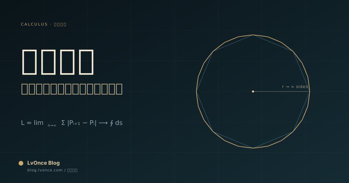
Calculus is often saddled with a reputation for being "profound," but strip away its formulaic garb and the kernel it lays bare usually comes down to a single idea—turning the curved into the straight. The curved is the world of continuous change; the straight is the world of the discrete and the computable. All that calculus does is build a bridge between the two, letting us approximate the curved with the straight, describe motion through stillness, and grasp the infinite through the finite.
"At a small enough scale, the world is always flat."—this is the greatest gift calculus gave to science.
Figure 1: Magnify the short curve segment inside the red box on the left, and the gap between arc and tangent shrinks to near-invisibility—this is the visual evidence of "local linearity."
1. The Core Idea of Turning the Curved into the Straight
Standing on the ground, you never feel that the Earth is round; walking a kilometer, you never sense the change in longitude. This is not dullness of the senses but an objective fact of local linearity: any sufficiently smooth surface, once you get close enough, reveals a face indistinguishable from a plane.
Calculus distills this plain intuition into a two-step strategy:
Divide and cut
: slice the curved, the changing, and the irregular into countless tiny segments.
Replace the curved with the straight
: on each tiny segment, substitute a straight line, a constant, or a linear approximation for the original curvature.
Replacing an arc of the curve y = f(x) over the interval [x,\,x+\Delta x] with a straight line incurs an error of roughly o(\Delta x). As \Delta x \to 0, the total error accumulated over the whole span is still a quantity of order zero:
This guarantees that "replacing the curved with the straight" is not a makeshift trick but a rigorous, reliable method. Below we walk through four derivations, moving from the most concrete circle to the most general curve, to show step by step how this idea works.
The Squeeze Theorem: Error Vanishing from Both Sides
"Replacing the curved with the straight" necessarily carries an error—a straight line is, after all, not a curve. On what grounds do we believe this error truly vanishes as n \to \infty? The answer is the Squeeze Theorem.
Suppose we have three sequences a_n, b_n, c_n, satisfying a_n \leq b_n \leq c_n for all n. If both ends a_n and c_n converge to the same limit L, then the b_n trapped in the middle has no choice but to converge to L as well:
Translated into the language of "turning the curved into the straight": to pin down the length, area, or some unknown "true value" T of a curve, we need not attack it head-on; we need only construct two approximations that converge to the same limit—
one
approaches from below
T
, written
L_n⁻
, always less than or equal to the true value;
one
approaches from above
T
, written
L_n⁺
, always greater than or equal to the true value;
when the gap
L_n⁺ − L_n⁻ → 0
, the trapped
T
is hemmed in from both sides and uniquely determined.
The geometric intuition of the Squeeze Theorem: the upper and lower sequences are like two closing doors that press the true value onto the single point L.
This is exactly the essence of Archimedes' "method of exhaustion" from over two thousand years ago, and also the very definition of the Riemann integral. Each of the four derivations below can be read as a concrete enactment of the Squeeze Theorem—inscribed (lower bound), circumscribed (upper bound), or lower sum and upper sum—squeezing the true value out from both sides.
2. Deriving the Circumference of a Circle
The circle is the most perfect of curves—curved everywhere, symmetric everywhere. How do we measure its length? The Greek Archimedes gave the plainest answer: approximate it with regular polygons made of straight lines.
Strategy: The Inscribed Regular n-gon
Draw a regular n-gon inside a circle of radius r. The distance from the center to each vertex is r, and the central angle subtended by two adjacent vertices is \theta = \frac{2\pi}{n}.
Figure 2: As the number of sides grows, the polygon's broken boundary hugs the circular arc ever more closely.
The Derivation
Step 1: Find the length of a single side. Two adjacent vertices together with the center form an isosceles triangle whose base (one side of the regular polygon) has length:
Figure 3: A single triangular element—central angle θ = 2π/n, base length l = 2r sin(π/n).
Step 2: The perimeter of the regular n-gon is the sum of n sides:
Step 3: Let n \to \infty. Set t = \pi/n, so t \to 0, and use the fundamental limit \lim_{t \to 0}\frac{\sin t}{t} = 1:
The circumference of the circle equals 2\pi r. The "straightening" of the broken line becomes an exact equality in the limit n \to \infty.
The Squeeze Argument: Inscribed and Circumscribed Closing In from Both Sides
Above we used only the inscribed polygon ("propping up from inside"), which gives a lower bound for the circumference—because a chord is shorter than its arc. But equally natural is the circumscribed regular n-gon: each side is tangent to the circle and wraps it from outside, giving an upper bound. Together they form an Archimedean squeeze:
Each side of the circumscribed regular n-gon has length 2r\tan(\pi/n), so P_n^{\text{out}} = 2nr\tan(\pi/n). Setting t = \pi/n, by the fundamental limit \tan t / t \to 1:
The lower bound P_n^{\text{in}} \to 2\pi r and the upper bound P_n^{\text{out}} \to 2\pi r; by the Squeeze Theorem the circumference C is uniquely determined to be 2\pi r. This is precisely how Archimedes estimated π over two thousand years ago—he doubled from n=6 all the way to n=96, obtaining the precise range 3\tfrac{10}{71} < \pi < 3\tfrac{1}{7}. The error vanished not because of "a good guess" but because it was wiped out by hand by the geometric lower and upper bounds on both sides.
The circle is trapped between two layers of polygons: the inscribed (green) props it up from inside, the circumscribed (red) presses down from outside; as n grows, the gap between the red and green rings closes at a rate of 1/n², and the circumference is locked in as 2πr.
3. Deriving the Area of a Circle
Once we know the circumference, the area is not far off. The method is again "cutting into straight elements."
Strategy: Slice the Circle into n Triangles
Draw lines from the center to n equally spaced points, dividing the circle into n congruent isosceles triangles. The base of each triangle is one side of the regular polygon, and its height is the distance from the center to that base (the apothem).
Figure 4: Cut the circle into many triangles; arranged alternately, they nearly assemble into a rectangle of width πr and height r.
The Derivation
Step 1: Each triangle has base 2r\sin\frac{\pi}{n} and height (the perpendicular distance from the center to the base) r\cos\frac{\pi}{n}.
Step 2: The area of a single triangle:
Step 3: The total area of n triangles:
Step 4: Let n \to \infty and set u = 2\pi/n:
The area of the circle equals \pi r^2. Note the elegant relation with the circumference: A = \frac{1}{2} \cdot C \cdot r = \frac{1}{2} \cdot 2\pi r \cdot r—the area equals "half the circumference times the radius," just like the area of the rectangle you get by cutting the triangles open and laying them flat.
The Squeeze Argument: Areas of the Inner and Outer Polygons
Likewise, the inscribed and circumscribed regular n-gons furnish a natural lower and upper bound for the circle's area—the inscribed polygon lies entirely inside the circle, the circumscribed polygon entirely encloses it:
The circumscribed regular n-gon can be seen as n isosceles triangles assembled together, each with base 2r\tan(\pi/n) and height r, so A_n^{\text{out}} = nr^2\tan(\pi/n). Setting t = \pi/n:
The lower bound A_n^{\text{in}} \to \pi r^2 and the upper bound A_n^{\text{out}} \to \pi r^2 meet at the limit. By the Squeeze Theorem, the trapped \pi r^2 is the true area of the circle. Intuitively: the inner polygon "bulges" out from inside, the outer polygon "presses" down from outside; the larger n is, the narrower the gap, and the circle's area has nowhere to hide.
The orange annulus is exactly "upper bound − lower bound"—as n grows, its area shrinks to zero at O(1/n²), and the true area πr² of the circle, trapped in the gap between the two layers of polygons, has nowhere to escape.
4. Deriving the Arc Length of a General Curve
The circumference of a circle is a special case; for an arbitrary curve y = f(x), the strategy of "turning the curved into the straight" is exactly the same—slice the curve into countless tiny segments and replace each with a straight line.
Strategy: The Infinitesimal Right Triangle
Take two points (x,\,f(x)) and (x+dx,\,f(x+dx)) extremely close together on the curve. The arc length dl between them is approximately equal to the length of the segment joining the two points. And this segment is the hypotenuse of a right triangle:
Figure 5: A curve element—the horizontal dx and vertical dy form the legs, and the hypotenuse dl is the "straight-for-curved" approximation of that small segment.
The Derivation
Step 1: By the Pythagorean theorem, the arc-length element is:
Step 2: Sum all elements for the curve y = f(x) from a to b:
Example: Find the arc length of the parabola y = x^2 over [0,\,1]. Here f'(x) = 2x, so:
Slightly longer than the straight-line distance \sqrt{2} \approx 1.414—precisely the extra path introduced by the curve's "bending."
Figure 6: Take 4 equally spaced points on [0,1] and connect them with a polyline; its total length approaches the arc-length integral ≈ 1.4789 as the number of segments increases.
The Squeeze Argument: Polyline Length (Lower Bound) and Sum of Tangent Segments (Upper Bound)
How do we rigorously show that "the finer the subdivision, the closer the polyline length gets to the true arc length"? Again by the Squeeze Theorem, trapping the arc length L from both sides.
Lower bound—the inscribed polyline: Divide [a,b] into n segments and connect adjacent division points with chords. "Between two points the straight line is shortest," so each chord is no longer than the corresponding arc. Summing all chords:
Upper bound—the sum of tangent segments: Suppose |f''| \leq M. At the endpoint x_i of the i-th segment draw the tangent, and take the position \eta_i where the absolute slope is largest on that segment; then this arc can always be covered by a "longest projection" of length \sqrt{1+[f'(\eta_i)]^2}\,\Delta x along the tangent direction:
The two ends meet: By the Lagrange Mean Value Theorem, each chord satisfies \Delta y_i = f'(\xi_i)\,\Delta x (\xi_i \in (x_{i-1}, x_i)), so L_n^- = \sum \sqrt{1+[f'(\xi_i)]^2}\,\Delta x. As n \to \infty, both L_n^- and L_n^+ are Riemann sums of the same integrand \sqrt{1+[f'(x)]^2}, and their gap—controlled by the uniform continuity of f'—tends to zero:
By the Squeeze Theorem, L equals this integral. Worth savoring: in Section 2 we trapped the circumference with two sets of polygons—"inscribed" plus "circumscribed"; here we switch to "chord polyline" plus "tangent segments," two sets of broken lines trapping a general arc length—different in form, identical in structure.
The same arc (blue) is trapped from both sides by two sets of broken lines: on the left, the green chord polyline connects adjacent division points, each chord shorter than its arc, summing to a lower bound; on the right, the red tangent segments extend along the curve's tangent at each segment, each longer than its arc, summing to an upper bound. As the subdivision is refined, both converge to the same integral value.
5. Deriving the Area of a General Region
The same idea of "turning the curved into the straight" can be used to find the area beneath a curve. This time we replace the "curved" boundary with "straight" rectangles.
Strategy: The Riemann Sum
Partition the interval [a,b] into n equal parts, each of width \Delta x = \frac{b-a}{n}. On each subinterval erect a rectangle whose height is a function value from that interval.
Figure 7: On the left, rectangle heights take the left endpoint (lower sum, area too small); on the right, they take the right endpoint (upper sum, area too large). Both squeeze to the same limit.
The Derivation
Step 1: Define the lower sum (taking the left value of each segment) and the upper sum (taking the right value):
Step 2: When f is continuous on [a,b], the difference between the upper and lower sums:
where \omega(\Delta x) is the maximum oscillation of f within a width \Delta x; the uniform continuity of a continuous function guarantees it tends to zero.
Step 3: By the Squeeze Theorem, s_n and S_n converge to the same limit, which is the definite integral:
Example: Find the area enclosed by y = x^2 over [0,1] and the x-axis. Partition into n parts and take the right endpoint:
So \int_0^1 x^2\,dx = \frac{1}{3}. The area of the curvilinear trapezoid is approximated by the "straight" areas of countless rectangular strips.
6. From Special to General: A Unified View of Turning the Curved into the Straight
Looking back at the four derivations above, the pattern is strikingly consistent:
Circumference of a circle
: sides of a regular polygon → circular arc (a straight line approximating a curve)
Area of a circle
: assembled triangles → circular region (a straight-edged figure approximating a curved one)
General arc length
: Pythagorean elements → arc (a generalization of 1)
General area
: rectangular strips → curvilinear region (a generalization of 2)
Going further, viewed through the lens of vanishing error, they also share the same squeeze skeleton—one can always find a slightly-too-small lower bound and a slightly-too-large upper bound, leaving the true value nowhere to escape:
True value | Lower bound (too small) | Upper bound (too large) |
|---|---|---|
Circumference 2πr | Inscribed polyline 2nr sin(π/n) | Circumscribed polyline 2nr tan(π/n) |
Area πr² | Inscribed polygon area | Circumscribed polygon area |
Arc length L | Inscribed polyline length | Sum of tangent-segment lengths |
Definite integral ∫f | Lower sum s_n | Upper sum S_n |
"Replacing the curved with the straight" provides the method for constructing lower/upper bounds, while the Squeeze Theorem provides the logical guarantee for why such a construction must converge to the true value—the former is intuition, the latter is evidence. Together they turn "at a small enough scale the world is always flat" from a slogan into a tool that can be used with rigor.
They all first "cut into pieces," then "replace the curved with the straight," and finally take the limit. Differentiation tears the whole into local straight lines; integration stitches countless straight lines back into the whole—this is the duality proclaimed by the Newton–Leibniz formula:
No matter how finely you cut, in the end you need only return to the difference at the endpoints. All the "straight-for-curved" approximations are perfectly absorbed in the summation.
7. Why the Upper and Lower Bounds Are the Truth—The Plain Logic of Decomposing Complexity
Having read this far, one question may still linger: why must "upper bound equals lower bound" equal the truth? What if the truth were some "third value" we have not yet noticed, lying outside the two? This seemingly philosophical doubt is in fact answered most deeply by the completeness of the real numbers—the very foundation on which the entire edifice of advanced mathematics stands.
1. Completeness: There Are No Gaps on the Real Line
When we say L_n^{-} \leq T \leq L_n^{+} and L_n^{+} - L_n^{-} \to 0, we are essentially placing on the number line a series of nested intervals [L_n^{-},\,L_n^{+}], each containing the next, with lengths tending to zero. The completeness axiom of the reals (also known as the nested interval theorem) guarantees that such a nest of intervals has one and only one common point.
"Only one" is the key. If there were some "gap" on the real line, letting two distinct values T_1 \neq T_2 both be trapped, then there would be a nonzero distance |T_1 - T_2| > 0 between them—but this contradicts L_n^{+} - L_n^{-} \to 0. So "upper bound = lower bound" is, in the real number system, equivalent to "the truth is uniquely determined"—not a coincidence, but a property built into the reals when they were constructed.
2. The Three-Step Paradigm of Plain Logic
Abstracting the idea above, we obtain a unified decomposition template that spans every branch of mathematics:
Construct a lower bound
: find a slightly-too-small, easy-to-compute approximation
Lₙ⁻
("I am at least this much");
Construct an upper bound
: find a slightly-too-large, easy-to-compute approximation
Lₙ⁺
("I am at most this much");
Compress the gap
: let the difference between the two tend to zero as some parameter (
n
,
Δx
,
ε
) shrinks, and the truth is naturally squeezed out.
This paradigm recurs on almost every "hard-to-compute-directly" object in advanced mathematics:
The ε–δ definition of a limit
: to prove
xₙ → L
is essentially to construct an upper bound
L+ε
and a lower bound
L−ε
, trapping the sequence in an arbitrarily small ε-interval.
Construction of the reals (Dedekind cuts / Cauchy sequences)
: every irrational number is itself defined as an "upper/lower partition" of the rationals—it is precisely the unique new number that strictly separates the upper set from the lower set.
Riemann integrability
: a function is integrable ⇔ the upper and lower sums share a common limit. Integrability is just another name for "the squeeze skeleton does not collapse."
Extrema and optimization
: finding
inf
and
sup
—the infimum and supremum—is itself a two-sided squeeze on the true value.
Error estimation in numerical methods
: Runge–Kutta, finite differences, finite elements, Monte Carlo—each gives a convergent solution plus an error band in upper/lower-bound form; without "upper and lower bound estimates" there is no trustworthy numerical result.
Algorithmic complexity analysis
: when the asymptotic upper bound
O(·)
and lower bound
Ω(·)
hold simultaneously, they give a tight bound
Θ(·)
—this is the Squeeze Theorem of computer science.
3. Generalizing to Arbitrary Problems: Replace "Hard" with "Two Easies"
On a grander scale, "turning the curved into the straight + squeezing from above and below" offers a meta-method for problem-solving—when a problem is hard to attack head-on, replace it with two easy-to-handle approximations pointing in opposite directions, and let the true value emerge automatically between them:
Can't measure the length of a curve? Construct a short polyline (below) and long tangent segments (above), converging together.
Can't measure an area? Construct a lower sum (below) and an upper sum (above), converging together.
Can't find the exact value of
π
? Archimedes constructed inscribed (below) and circumscribed (above) polygon perimeters, converging together.
Can't prove an inequality directly? A common trick is scaling—enlarge the target to an easily proven upper bound and shrink it to an easily proven lower bound, squeezing the conclusion out from both sides.
Don't know the optimal solution of an NP problem? Give an approximation algorithm's solution (a lower-bound proof, "at least this good") plus a heuristic relaxation (an upper-bound proof, "cannot be worse"), squeezing out the feasible region of the optimum.
Facing fuzzy engineering metrics (response time, bit-error rate)? Give a worst-case upper bound plus a best-case lower bound, so the SLA is precisely characterized between the two.
The beauty of this approach lies not in being "clever" but in turning cognitive uncertainty into constructive controllability. We admit our direct knowledge of the truth is limited, but as long as we can keep approaching from both sides and compress the gap to arbitrary smallness, the truth is "forced out" by the process—not computed by us, but promised in advance to us by the completeness of the reals.
The whole decomposition logic of advanced mathematics can be condensed into one sentence: "Place the uncomputable object between two computable approximations." Turning the curved into the straight provides the "approximation"; the Squeeze Theorem provides the "legitimacy of the placement." The former is craft, the latter is contract.
From Archimedes' polygons to Newton's calculus, from Riemann's integrability to Shannon's information theory, from Monte Carlo simulation to the convergence of deep-learning loss functions—the way humanity decomposes the complex world has essentially always been the same: find a pair of approximations that will meet, and let the truth have nowhere to hide at their meeting point.
"Turning the curved into the straight" is far more than a mathematical trick; it is a universal cognitive strategy: Taylor expansions replace functions with polynomials, finite elements cut complex geometry into triangles, neural networks are the stitching together of countless local linearities... the entire industry of numerical computation is about carrying the "curved" world into the realm of the "straight" to be digested.
Anything sufficiently smooth can be treated as straight at a small enough scale; any sufficiently complex whole can be assembled from countless simple local pieces.
This is a plain kind of optimism—it believes complexity is never unsolvable, so long as one is willing to cut finely enough and add up enough pieces. Turning the curved into the straight is not merely a set of algorithms calculus gives us, but a posture for facing a complex world.